How to run?

Run 'cg_exe' - the band structure calculation by conjugate-gradient diagonalizationn

日本語

  Here the manual gives an example to explain how to run FPSEID²¹ code. This guidance is written for people who already made executable load modules. If you have not obtained 'cg_exe', 'sd_exe, and 'tddft_exe', go to How to compile?
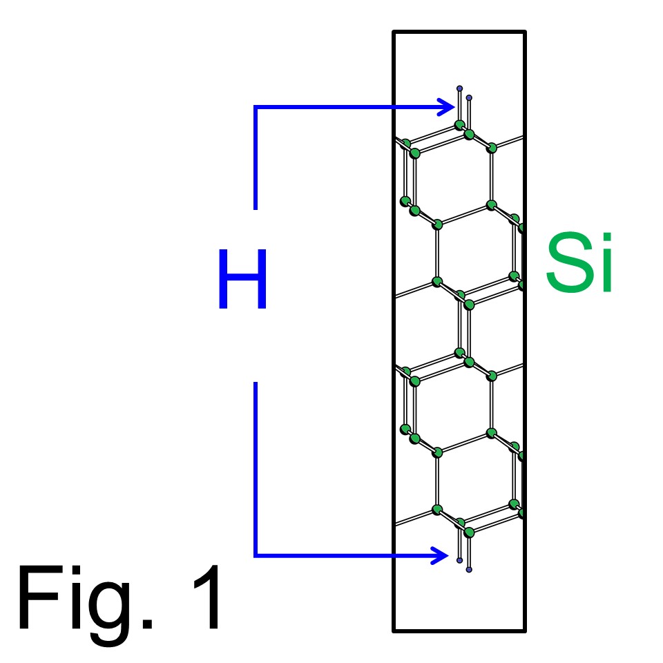
The example has a structure as illustrated in Fig. 1, which is a Si(111) slab model terminated by H atoms on top and bottom. Here the conventional band structure calculation is performed to make first-step toward the TDDFT calculations, which simulate laser-induced H desorption.
  Now this manual explains the 'first-step' running of 'cg_exe' needed for the TDDFT calculation. The structure shown in Fig. 1 has 1x1 periodicity in surface lateral directions and 12 atomic layer of Si exists in a slab. The shape of the unitcell is hexagonal. The input data named as 'Si111-H.in' is displayed inside a box below. Here, parameters requiring high attention are displayed as boldface which will be explained below the box. Other parameters should be remained as they are. (This template file is obtained from download 'Si111-H.in')

   In the first line, Si(111)1x1 H-term cell is just a title of subject. You can write anything to identify what you do.
From second line to the end of the header of the input data, all characters are case sensitive. Second line ALAT=4.4427103... is a lattice paramerte in Bohr radius. Please be careful since many DFT package uses angstrom unit but this is not the case here. In this example, the Si-Si bondlength in cubic Si crystal is given. (Not an experimental value)
 Again, in the second line, ZVAL=50 gives # of all valence electrons per unitcell. The system of Fig. 1 contains 12 Si and 2 H atoms, thus total number of valence electron per unitcell = 4x12 + 2 =50. (Note that the FPSEID²¹ package treats valence orbitals only within spin-unpolarized approximation.) RCUT=845 is a value needed for the Ewald summation and preferred to be longer than the longest lattice vector of the unitcell. (The unit is (Bohr radius)²) GCUT=12.0 means the cut-off energy of the plane-wave basis set to describe charge density and potential with the Rydberg unit.
   In the third line, CD=ATOM means that the calculation starts with initial guess of the valence charge density which is given by atomic pseudo-orbitals. (The pseudo-orbitals is taken from a file represent the norm-conserving pseudopotentials. The usage of pseudopotentials will be explained below.) WF=INIT means that the calculation starts with initial guess of the valence wavefunctions given by plane waves with single G vector. (Please note if the calculation is done by using previously obtained charge density and wavefunctions, you should set CD=FILE WF=FILE.) The label CG in this line is necessary and should be changed when we run 'sd_exe' which will be explained later.
  In the fourth line, METAL=(25,0) means, number of occupied bands is 25, and number of metallic bands is 0. (The metallic band means the bands crossing the Fermi level.) In the FPSEID²¹ package, only valence orbitals are treated within spin-unpolarized approximation. The system of Fig. 1 contains 12 Si and 2 H atoms, thus total number of valence electron per unitcell = 4x12 + 2 =50. Thus, the number of all occupied band per spin is 25. One can be interested in cases of metallic systems, which needs some trick and will be explained when contacted through Inquiry. In the same line, FFTWF request the Fourier transformation of wavefunction from the G-space to the real-space, that will be used to run 'sd_exe' to expand wavefunctions in full-grid G-space.
   The fifth line CONV=1.D-7 gives conversion criteria of the self-consistent potentials. (This value will be increased into 1.D-5, when running 'tddft_exe' for practical efficiency. Note that this line ended with '/' which indicates the end of the header.

   Below the headlines, the first three lines indicate Cartesian coordinates of lattice vectors (A1-A3 vectors). All elements of A1-A3 vectors are multiplied by a value of ALAT at running the code.
   Below the lattice vectors, '2 Si12H2' is denoted. The code actually read '2' only which is a number of atomic type in the unitcell. In this example, there are two kinds of atoms (Si and H).
   Next line describes Si atoms and 12  2  28.0855 respectively describe # of Si atoms, # of pseudo-orbitals for the norm-conserving pseudopotentials, and atomic mass in unit of mass of proton. In Si case, the pseudopotentials have Si 3s and 3p components, thus the # of pseudo-orbital is 2. (In case of Cu, the # of pseudo-orbitals is 3, Cu 4s, 4p, and 3d components. Meanwhile, in case of C, the # of pseudo-orbitals is 1, C 2s component. Note that the C 2p component is not used.) Then following 12 lines are atomic coordinates of Si atoms in unit of A1-A3 vectors.
   Next line describes H atoms and -2  0  1.0 respectively describe # of H atoms, # of pseudo-orbitals for the norm-conserving pseudopotentials, and atomic mass in unit of mass of proton. It is strange that number of atoms is given in negative one but it is only in cases of H and He in which pseudopotentials are given as local potentials (no need to use pseudo-wavefunctions for nonlocal part). This strange rule is historically given linked with '0' for # of pseudo-orbitals and validation in using positive number has not been checked. Then following 2 lines are atomic coordinates of H atoms in unit of A1-A3 vectors.
After atomic coordinates of H atoms, the next coming lines represents k-vector mesh points used in the calculation.
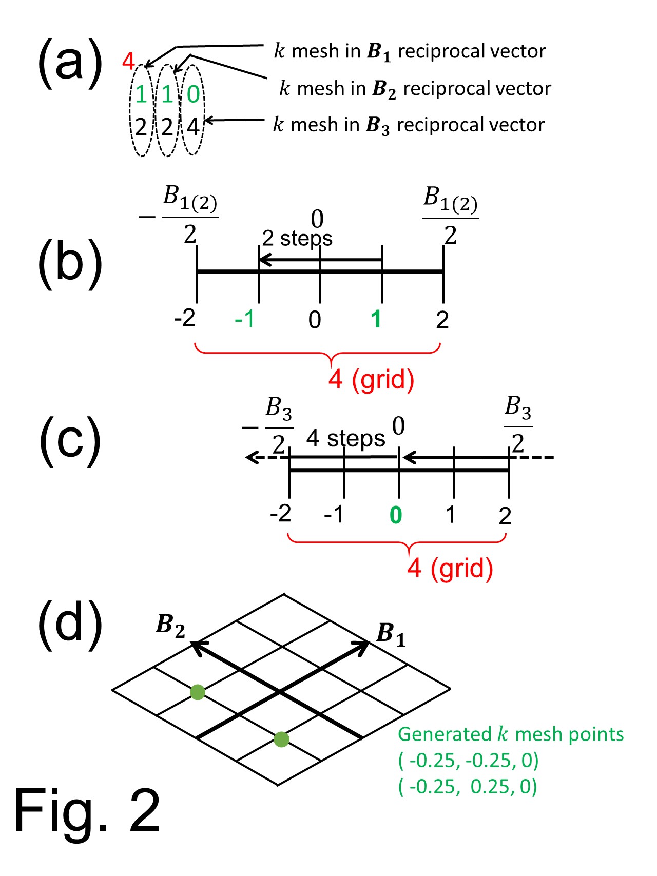In the 'Si(111)-H.in' data shown in above box, there is
 4
   1  1  0
   2  2  4
Here, the top number 4 defines grid # of k-vector in all reciprocal vectors. Thus, each reciprocal vector (here called as B1 B2 B3 vectors) has grid points from -2 to 2 as shown in Fig. 2 (b) to divide one of reciprocal vector into four pieces. The second line   1  1  0 denotes the starting point to generate the k-point and each number links to the number directly below, as shown in Fig. 2 (a). The third line   2  2  4 show steps to move one grid to neighbor, as shown in Fig. 2 (b) for B1 B2 vectors and in Fig 2 (c) for B3 vector. In this manner, grid point for each reciprocal vectors generated as shown in green-colored numbers in Figs. 2 (b) and (c). Finally, the generated grid points of all reciprocal vector are used to generate k-points in the first Brillouin zone. Fig. 2 (d) shows the current case in which the k point has zero component in B3 vector. Note that the current case has no spin-orbit interaction thus there is degeneracy between Block state with vector k and -k, thus the irreducible k-points is two.
  The bottom two line shows electron occupation on each atomic valence orbitals for Si and H. The Si 2s and 2p orbitals respectively have 2 elecrtons, while H 1s and 2p orbitlas has 1 and 0 electrons. (The case H atom may sounds strange but currently employed pseudopotential do not referr the orbitals with the same angular momentum.) Here is not the case of Cu which has 3d. 4s (and 4p) orbitals as valence electrons. But Cu case needs to define the occupation number as 1.0 0.0 10.0 as current format orders pseudo-wavefunctions and pseudopotentials in increasing order of the angular momentum, thus 4s, 4p and 3d.
  Besides the 'Si111-H.in' file, there are files for input data as 'size.dat', 'sym.C1' and pseudopotentials. All of these have specific contents suitable only to FPSEID²¹ package.
  The 'size.dat' which is an asci file with free-format, gives necessary size of arrays used in FPSEID²¹ package which is genrated by following procedure.he contents of 'size.dat' for this example is as follows with explanations:
  Here, ways to determine each number in 'size.dat' are explained. From input data, we can give immediately the # of irreducivle k-points, # of occupied and empty states, and # of atoms and atomic types. Meantime, (NRX, NRY, NRZ) and (NG, NG2) are obtained by following equationns

rGcut=sqrt(Gcut)
Gnum=(2*rGcut)**3*Vol/(6*pi**2) * 1.25d0
Gnum2=Gnum/8.d0
NG=Int(Gnum)
NG2=Int(Gnum2)

Here, 'rGcut' means the cutt-off energy explained above.'Vol' means the volume of the unit cell in Bohr³ unit.

The FFT grid (NRX, NRY, NRZ) are obtained as following procedure

A1leng=ALAT*sqrt{ A1(1)**2 + A1(2)**2 + A1(3)**2 )
NRX=int(2*A1leng*Gcut/pi+1.d0)
A2leng=ALAT*sqrt{ A2(1)**2 + A2(2)**2 + A2(3)**2 )
NRY=int(2*A2leng*Gcut/pi+1.d0)
A3leng=ALAT*sqrt{ A3(1)**2 + A3(2)**2 + A3(3)**2 )
NRZ=int(2*A1leng*Gcut/pi+1.d0)

Then rechoose NRX NRY NRZ to be near ODD numbers, but the'Prime numbers' should be avoided for the efficient FFT performance.

  The file 'sym.C1' repersent that the calculated system has not symmetry and represent the identity matrix. The format is specific for FPSEID²¹ so it is recommended to obtaini this from sym.C1,

Here is an example of a script file to run 'cg_exe' which should be dependent on your Linux environment.　One can see assignment for files at FORT41, FORT46, FORT42. (For 'Aurora' users, please use VE_FORT41, VE_FORT46, VE_FORT42 for file I/O settings.) These files are norm conserving pseudopotentials obtained by a scheme [N. Troullier and J. L. Martins, 'Efficient pseudopotentials for plane-wave calculation', Phys. Rev. B43, 1993 (1991)]. The pseudopotentials are in asci code, and downloadable from the box of the script below. Here, the manual recommends to create 'TR' directory on your account to store pseudopotentials in order to match with this script. Generally, the I/O number for the i-th type atom' (not the i-th atom) pseudopotentials is given 40+i when the atomic type corresponds to light elements, from H to Ne. On the other hand, when the i-th type atom corresponds to heavier elements, the pseudopotential files are separated into two with the I/O number 40+i and 40+i+5. This is very specific format and fits to FPSEID²¹ only. Note i-th atom's pseudopotential files with their names ending asr 'g.asci' or 'g.asc' should be used with I/O # 40+i. Meanwhile, file names ending as 'e.asci' or 'e.asc' should be used with I/O number 40+i+5. Indeed, one can confirm that rule in the following script, Pseudopotentials for Si and H atom can be downloaded when you click corresponding one displayed in a box below.
When 'cg_exe' is performed, output files (binary) 'rh.Si111-H_new','wf.Si111-H_new', and 'wf_real.Si111-H_new' are generated. So please reneme 'rh.Si111-H_new as 'rh.Si111-H, ,'wf.Si111-H_new' as ,'wf.Si111-H', and 'wf_real.Si111-H_new' as 'wf_real.Si111-H'. Then, please check that the calculation reaches the SCF solution by typing
$ grep ITR Si111-H.out
to see whether convergency criterion is satisfied. If not, restart 'cg_exe' by changing the header of input file 'Si111-H.in' as follows; 'CD=ATOM' should be 'CD=FILE' and 'WF=INIT' should be 'WF=FILE. Then confirm the SCF congergency and rename all '*_new' files to those without the tail '_new'.'
 The next step is running 'sd_exe'. To run 'sd_exe', visit manual for 'sd_exe'
One can also obtain the output file 'Si111-H.out' (asci) which is downloadable in above box. Here, description of some essencial parts is given.in red font as below.

Run 'sd_exe' - the band structure calculation by steepest-descent diagonalization

Run 'tddft_exe'- the electron-ion dynamics under laser field