Demo of Preprocessing
BIDO can perform the following sorts
of data preprocessing as part of array data (or huddle data) analysis.
1) Removal of trends
(direct-current components)
In
case the waveform baseline drifts linearly with time, removing its influence
may help to extract a larger number of segments for use in spectral analysis,
and to do so more appropriately.
2) Tapering of waveforms
A
preprocessing to be applied prior to bandpass
filtering that makes the waveform amplitudes converge more smoothly toward zero
near both ends.
3) Bandpass
filtering
Cutting
off noise-rich frequency bands by filtering may help to extract a larger number
of segments for use in spectral analysis, and to do so more appropriately.
4) Data decimation
This
helps to reduce the time it takes to do spectral analysis. Decimation cuts
high-frequency bands off the data, but it does not affect the accuracy of
analysis in the analyzable frequency bands.
5) Correction for
differences in instrumental characteristics
Data
from a recording system, where instrumental response characteristics differ
from channel to channel, are not immediately suitable for array analysis. They
may turn into usable array data when the differences in instrumental
characteristics are corrected for.
Those
who are using BIDO for the first time are requested to read Demo of array data analysis first in order
to get familiar with its general usage. Here we explain the preprocessing part
by using the demo data in \demo\HDL0002, which were made available by courtesy
of Dr Tatsuya Noguchi of Tottori University, just as was the case with
\demo\HDL0001 (see Demo of a huddle test
for descriptions of HDL0001). They were recorded on the same day and under the
same environment as HDL0001, except for differences in the sensor locations as
shown in the photos below.

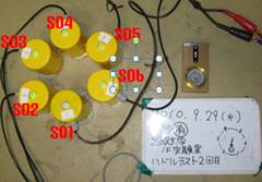
HDL0001
HDL0002
Please start the analysis
by typing
run.sh demo/HDL0002/param.sh [RETURN KEY].
You will be asked in a
dialogue, "Preprocessing the data?" Answering "y" (for yes)
allows you to apply preprocessing to the data. If you use the default answers
to all the questions in this demo, you will first encounter the following plot
of waveforms. These are the original data before preprocessing.

Please be sure to take a
look at
important messages that will be given at this stage in the dialogue:
-------------------------Citation
begins here-------------------------------
Do you want to preprocess
the waveforms? [y/n]
[This includes
elimination of the trend, application of tapers (and bandpass
filtering and decimation if necessary)]
NOTE: The original data
will be moved to a directory named "originaldata",
which will be automatically created by BIDO under the directory where the
original data files are currently stored. Instead, new files with the same
names as those of the original data will be created to store the preprocessed data.
(The seismfile will also be moved to the directory
"originaldata" as well, and newly created
by BIDO under the directory where the original seismfiles
are currently stored. This is necessary because the preprocessing possibly
involves decimation.) The original data files will not be overwritten
(destroyed) by BIDO. It is strongly recommended, however, to create backup of
the original data files to avoid their accidental destruction.
Type "n" to
skip preprocessing.
-------------------------Citation ends here-------------------------------
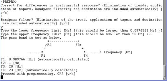
Typing "y" here launches a
dialogue for implementing the preprocessing. Answer "n" to
"Correct for the difference in instrumental response?" and
"y" to "Bandpass filter?"
(corrections for the differences in instrumental response will be explained
later). Setting the cutoff limits on the low- and high-frequency sides at 1 and
20 [Hz] respectively, you will see a message, asking for final confirmation, as
follows:
Type
"y", and you will see the preprocessed waveforms as follows. Bandpass filtering has eliminated the undulations
(components of long periods on the order of tens of seconds) that the original
data contained.

The
application of a bandpass filter automatically
involves the elimination of trends, tapering and decimation. The taper is of a
cosine type and is applied, by default, to 5% parts on both ends of the waveforms.
The length percentage of tapering can be modified through the variable tpend in \script\setpar.sh. Bandpass
filtering uses a Chebyshev filter I with an equiripple passband as described
by Saito (1978). After filtering, the data are decimated automatically (to a
maximal extent) by considering the cutoff on the high-frequency side. In the
present analysis, the sampling time interval is 0.01 sec in the original data,
but high-frequency ranges in excess of 20-23 Hz have been discarded through
filtering. Therefore, the data are decimated so as to reset the sampling time
interval at 0.02 sec, or to reset the Nyquist
frequency at 25 Hz.
Let
us check out what files there are beneath \demo\HDL0002. The folder is made up
as follows:
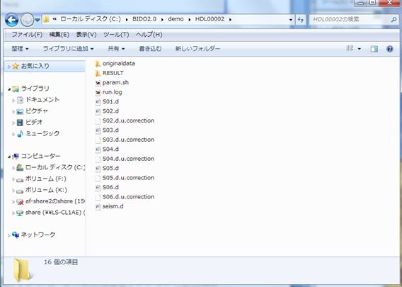
You
will see that a folder, named originaldata, has been
generated as was so indicated in the dialogue message. Please note that all
original data files have been moved there, whereas all data files that you find
here, named S0X.d, are preprocessed data (the same thing is true for seism.d).
When
the preprocessing is over, you will again see the message
Do
you want to preprocess the waveforms? [y/n]
in
addition to graphic output of the waveforms. Type "n", and you can
proceed to the next stage, or the main part of the analysis. You can repeat
preprocessing as many times as you like by typing "y". All
repetitions that follow proceed along the line: i)
Reading of the original data stored in the folder originaldata;
ii) Preprocessing, and iii) Output to the data folder (the preprocessed
waveform data files are overwritten). Therefore, the data will return to their
original state if you answer "n" (not to apply) to all preprocessing
options during the dialogue.
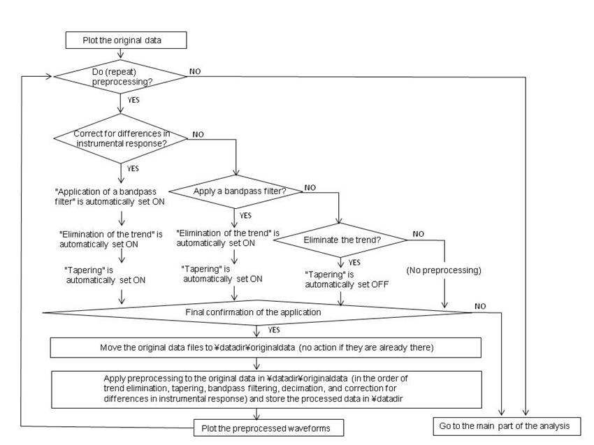
The
flow of preprocessing by dialogue can be summarized as follows:
Correction
for differences in instrumental characteristics
In the analysis results for HDL0002,
you may have noticed that the phase characteristics of channel no. 3 (data file
S03.d) behave differently than those of the other channels, just like in the
case of the analysis results for HDL0001 (see the analysis results in the Demo of a huddle test). It appears that
channel no. 3 tends to respond differently than the other sensors. When, like
in this case, the recording characteristics of a particular channel always
demonstrate an identical bias (or peculiarity) irrespective of who installs it
(or slight differences in the circumstances of installation), it appears
sensible to correct for the difference before proceeding to the data analysis.
BIDO is capable of implementing such corrections.
Create a file, in the folder where
the data files are stored, which helps to correct for differences in the
instrumental response characteristics, one for each seismic sensor component.
The files should be named like:
(data file name).{e, n,
u}.correction
where e, n and u correspond to the
east-west, north-south and up-down components, respectively. The five files in
the HDL0002 archive, named "*.u.correction,"
are the files for correction. Each file contains the following data strings:
Frequency F [Hz} Amplitude ratio R
[non-dimensional] Phase
difference P [deg]
If the FFT spectrum of the
pre-correction data is given by A exp(iq), the post-correction spectrum will
be (A/R) exp(i(q-P)).
The frequency steps in the correction files can be anything (they are
interpolated linearly). R=1 and P=0 are postulated when no correction file
is found in the same folder even though the instrumental response
characteristics correction option is set ON.
Correction
files are already bundled together in the folder \demo\HDL0002. These
correction files are the analysis results from HDL0001, or \RESULT\ave\DIFINSTRES1 Xu.d, copied and
renamed \S0X.d.u.correction. Let us use these HDL0001 results to correct the
HDL0002 data before proceeding to analysis.
Restart
the analysis by typing
run.sh demo/HDL0002/param.sh [RETURN KEY].
Continue with the dialogue, and
answer "y" to "Do you want to preprocess the original waveforms
anew?" and "y" to "Correct for the difference in
instrumental response?" Preprocessing automatically involves bandpass filtering. Therefore, if you set the cut-off
limits on the low- and high-frequency sides at 1 and 20 [Hz] respectively, you
will see the following message asking for final confirmation:
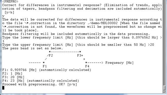
You
can proceed with preprocessing by typing "y". After a plot of the
waveforms, you will be asked again, "Do you want to preprocess the
original waveforms anew?" The differences in instrumental response have
already been corrected for, so type "n" to proceed to the main part
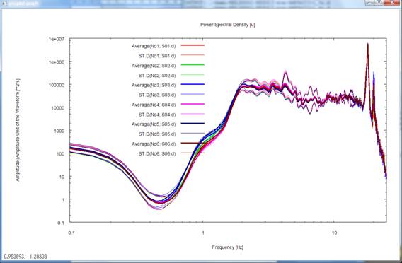
of the analysis. You will get the following final analysis results:
-
Power-spectral densities
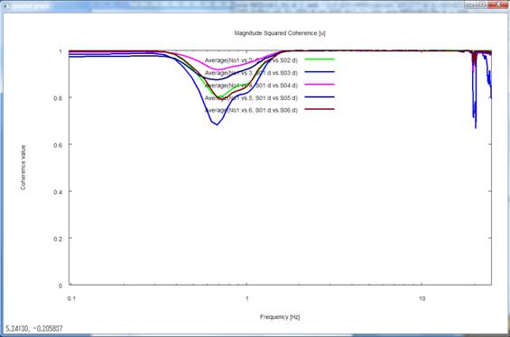
-
Magnitude-squared coherences
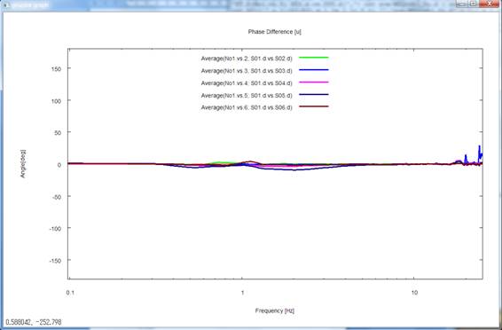
-
Phase differences
-
Noise-to-signal ratios

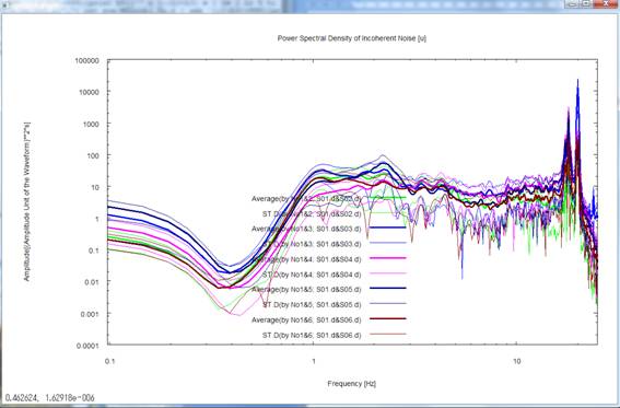
-
Power-spectral densities of incoherent noise
You
will notice the near-total disappearance of the peculiarity in phase
characteristics of channel no. 3 (data file S03.d) thanks to the correction for
differences in instrumental characteristics.
Saito,
M., 1978, An automatic design algorithm for band selective recursive digital
filters (in Japanese), Butsuri-Tanko (Geophysical
Exploration), 31, 112-135.