Demo of a Huddle Test
A
huddle test refers to a test where you huddle all seismic sensors at a single
location and record data simultaneously for the purpose of confirming the
agreement of the instrumental properties of all recording systems. In a huddle test, you can use exactly the same
analysis method that is described in the demo of
array data analysis, so please read that page first if you are using
BIDO for the first time. You can conduct analysis following exactly the same
procedure as in array analysis if only you assign identical locations to all
seismic sensors in the seismfile.
For example, please
download the demo data meant for huddle data analysis, decompress it beneath
the BIDO 2.0 folder, and analyze it following the same procedure that you would
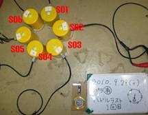
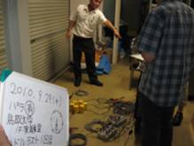
use to analyze array data. The demo data have been made available by courtesy
of Dr Tatsuya Noguchi at Tottori
University. They were obtained by six vertical motion sensors (HS-1
Geophones) of Oyo Geospace
Corporation installed on a concrete laboratory floor on the premises of
Tottori University (see photos), and were recorded by an es8 data recorder via
SA16 amplifiers and a low-pass filter (cutoff frequency 30 Hz).
Let us move on to data
analysis by typing
run.sh demo/HDL0001/param.sh
[RETURN KEY].
Just like in array
analysis, the analysis results are stored in a folder, named RESULT, that is
generated beneath the data folder.
The graphic output of the
huddle test includes:
- Power-spectral densities

- Magnitude-squared coherences

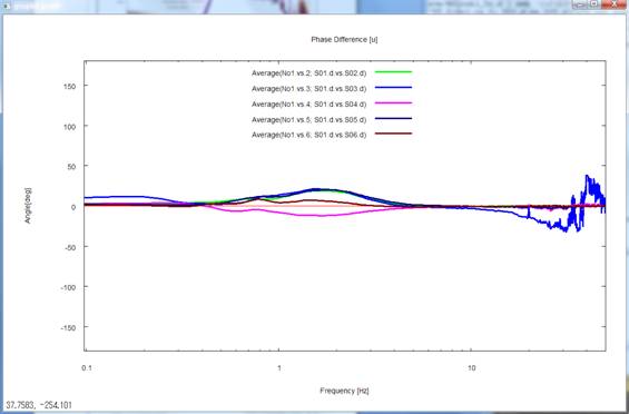
- Phase differences
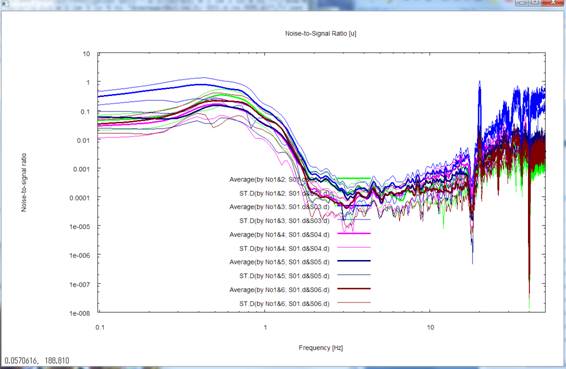
- Noise-to-signal ratios
and
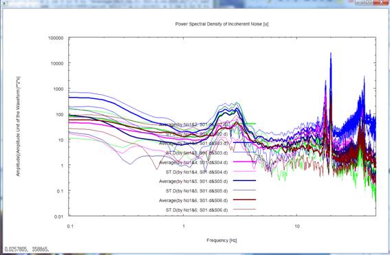
- Power-spectral densities of incoherent noise.
All graphic output is shown up to the maximum
frequency with the frequency axis scaled logarithmically. The maximum frequency
here refers to the smaller one between the value set by the parameter
freqmax_ave in \script/\setpar.sh (50 Hz by default but modifiable on your own)
and the Nyquist frequency. If you do not prefer logarithmic scaling, comment
out the line containing the parameter autologscale_x in \script/\setpar.sh by
appending # to the head of the line.
The legends for the magnitude-squared coherences
and phase differences are denoted like Average (by No 1 .vs. 2: S01.d .vs.
S02.d). This refers to the mean of coherences between record numbers 1 and 2,
of their phase differences (positive when 2 is more advanced than 1 in phase),
and of NS ratios and noise intensities calculated on their basis. Record number
1 refers to the data indicated at the top of the seismfile. The records are
numbered 2, 3 and so forth in the descending order of indication in the
seismfile from top to bottom. The letters "by No 1 .vs. 2" in the
graph legends indicate that record numbers 1 and 2 are concerned. To make this
point sure, these numbers are followed by data file names like "S01.d .vs.
S02.d." Please refer to ave.info in the ave folder for a table of
correspondence between the record numbers and file names. ST. D. means standard
deviation. The above analysis results show that record number 3 (records of
S03.d; blue) has distinctly low coherences and has large phase differences with
respect to the other records.
Bendat and Piersol (1971)
and Carter et al. (1973) are useful references for the estimation and physical
meaning of magnitude-squared coherences. The NS ratios are the inverse of the
SN ratios calculated by substituting the magnitude-squared coherences (coh2)
into the equation
![]()
(Carter et al., 1973). The
power-spectral densities of noise are calculated by multiplying the
power-spectral densities of the records by the NS ratios.
These plot data are
stored, as in the case of array analysis, in a folder named RESULT/ave. Please
refer to a list (here) of the file
names and descriptions of the plot data. There is a file named
DIFINSTRES1_2e.d. This file name is short for Differences in instrumental
response. It lays out the amplitude ratios and phase differences of record
number 2 with respect to record number 1 in the format
Frequency F [Hz] Amplitude ratio R
[non-dimensional] Phase
difference P [deg]
for each frequency. This
file, when renamed, can be used directly for the purpose of correcting for
instrumental characteristics in array data analysis (see Demo of data preprocessing).
Bendat, J. S.,
and A. G. Piersol, Random Data: Analysis
and Measurement Procedures: John Wiley & Sons, 1971.
Carter, G. C., C. H. Knapp, and A. H. Nuttall, 1973, Estimation
of the magnitude-squared coherence function via overlapped Fast Fourier
Transform processing: IEEE Transactions on Audio Electroacoustics, AU-21,
337–344.